
It’s the first day of week 3 of the SK Planet Busan Smart Port · Maritime Logistics Data Practice Course (K-New Deal Academy). Today’s topic was understanding data and data analysis. I heard that this Thursday I’ll actually analyze the monthly cargo volume trends at Busan Port. Today’s lecture was the groundwork laid before that.
Table of contents
Open Table of contents
- Data is already piling up everywhere
- An example starting from “15% drop in sales”
- Data, information, and insight are different things
- Two axes for dividing data
- The analysis process doesn’t flow in one direction
- Things that ruin analysis
- Three sentences that stuck with me today
- Things to study further
Data is already piling up everywhere
In daily life and at work, we encounter an enormous amount of data. Use an online shopping mall, and order history piles up. That same order history is a receipt to the buyer and a sales slip to the company. Agree to cookies, and your IP gets collected, revealing country and region, which gets used for marketing. Even the reviews left on a product we sold become data.
So there are three questions. What data fundamentally is, how to understand it, and how to analyze it to extract something useful.
An example starting from “15% drop in sales”
Say you run an online shopping mall. In the monthly report, you reported that sales dropped 15% this month.
Looking at the number alone, there’s exactly one thing you can tell: sales decreased. But you don’t know “why” it decreased.
This is where the definition of data analysis came in.
The process of defining a problem and collecting, organizing, and exploring relevant data to find evidence for the question.
It’s not a technique of computing numbers or drawing graphs — it’s interpreting the meaning the data reveals. We use pandas for analysis, but what stuck with me was that pandas only computes the numbers. The tool doesn’t do the interpreting for you.
Data, information, and insight are different things
Data is facts, numbers, symbols, and signals in an uninterpreted state. Things like a student’s exam score or a customer’s order amount. It has a value, but its meaning changes depending on context. Data isn’t a conclusion — it’s raw material to be interpreted in order to answer a question.
If all you have is “exam score: 85,” that’s just one fact. Add “10 points above the class average,” and now it has the meaning of having done well on the test. That’s information — the result of organizing data for a purpose and giving it context.
And what lets you connect information to an actual action is insight. Carrying forward the sales example, it looks like this.

You have to reach insight for it to help with decision-making. If you stop at “sales dropped 15%,” you can’t decide anything.
Two axes for dividing data
Data is divided along two perspectives. By form, it’s structured · semi-structured · unstructured. By character, it’s numerical · categorical.

The reason you need to look at both axes together is that you need to check both storage format and real-world meaning at the same time to choose an appropriate analysis method.
Classification by form
Structured Data — The position and meaning of each value is clear, and the same column repeats values of the same format. Each row is a single record, so it’s called a record, and each column represents a type of information a row can hold.
A schema is the blueprint for structured data that tells the computer how to process each value.
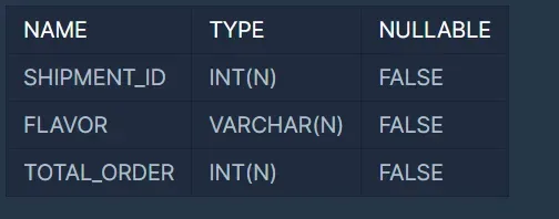
One important principle is that a single column should hold a single, consistent meaning. You shouldn’t cram everything into one cell like laptop/1 unit/1,200,000 won.
Structured data is organized in a way that makes it easy to extract insight, so it’s treated as high-value data.
Semi-structured Data — Instead of fixed rows and columns, keys, tags, and delimiters tell you the meaning and relationships of each value. It has metadata and can easily form nested structures. On the other hand, the structure can differ from record to record, so it needs to be processed once before analysis — things like unnesting, unifying data types, and unifying item names.
Unstructured Data — natural language, images, audio, video. Humans can understand it, but computer analysis requires separate feature extraction. This doesn’t mean the data lacks information — it means the meaning isn’t divided into explicit columns. Pixels and audio signals are arrays of numbers, but the meaning of the object, word, or action isn’t immediately apparent.
Humans can look at a photo and distinguish things right away, but you have to explicitly convey that distinction to a computer. So unstructured data can be converted into something structured-like by extracting features.
Classification by character
Numerical Data — Expresses quantity, size, degree, or measurement results as numbers, where operations like sum or average are meaningful.
- Discrete: Possible values are separated from each other, usually integer counts. Data you get by counting.
- Continuous: Possible values exist between any two values, and the recorded precision depends on measurement precision.
There’s a trap here: identifier data. Customer numbers, student IDs, phone numbers, and product codes look like numbers but don’t represent quantity or size. Averaging student IDs is meaningless.
For numerical data, you look at the center via mean, median, variance, and standard deviation, and look at distribution and relationships via histograms, box plots, and scatter plots.
Categorical Data — Instead of adding values, you compare how much falls into each category. So frequency and proportion matter. Combining two categorical variables into a cross-tabulation lets you see differences in distribution across groups.
- Nominal: Like blood type, region, color, or payment method — just different kinds, with no high or low.
- Ordinal: Like Bronze — Silver — Gold — Platinum, where you can compare which is higher.
When converting categories into numbers, the key is not creating an order that doesn’t actually exist.
| Type | Encoding | Reason |
|---|---|---|
| Nominal | One-hot encoding | No order exists, so each category gets its own independent column |
| Ordinal | Ordinal encoding | Order actually exists, so it can be expressed by magnitude |
Databases came up too. Membership tiers are often managed as stored codes, in which case you need to look at (JOIN) the membership tier ↔ stored code table together for it to have meaning.
The analysis process doesn’t flow in one direction
Data analysis isn’t about loading a file and computing right away — it’s a process of continually aligning the question, the data, and the method.

If you discover new facts during exploration or modeling, you go back to the question, collection, or preprocessing stages and revise them. Apparently going back actually happens quite often.
But there’s a condition attached. You must not keep expanding the problem. The original problem you set out to solve must never change, but adding necessary data or incorporating related data you discovered is fine. This was the line that struck me most today.
Problem definition
This is the stage where you decide what problem you’re trying to solve and what question the data will answer. In practice too, you start by setting a direction and then finding the problem.
The goal needs to be converted into an analysis question. A sentence that includes a time period, a metric, and a comparison is an analysis question. You need to fix the scope so you don’t wrongly compare different groups and periods mixed together. When setting the time period, you also need to set it so representativeness is secured.
A hypothesis is a tentative explanation you want to confirm with data. If the data doesn’t support the hypothesis, you need to accept that as is. The lecture also warned about confirmation bias — picking only the data that favors the hypothesis.
Data collection
Rather than gathering a lot, securing data with the scope and criteria that fit the defined question matters more. More isn’t necessarily better. If quality is low or there are many variables unrelated to the question, both processing cost and the chance of misjudgment rise together.
You need to align period, time zone, time point, unit, and aggregation criteria consistently to safely connect data together. And you need to check whether the collected data represents the whole. If the sample is skewed toward a particular group, it’s hard to generalize the same conclusion to the whole.
Preprocessing
Collected data is mixed with missing values, duplicates, and format inconsistencies, making it hard to analyze right away. Roughly three things are done.
- Check for missing values and outliers, remove duplicates
- Unify format, data type, unit, and category
- Create derived variables needed for the analysis purpose
First check for empty values and extreme values. They could be errors, but they could also be a signal of a specific group or an important event. 0 is likely to be an actually measured value, so you shouldn’t carelessly treat it as missing.
The example for format unification hit home immediately. If male · M · 남 are mixed together for gender, all three get counted as different values.
A derived variable is a variable that creates new meaning from original variables. If you have revenue and cost, subtract to create profit; if you have a reference date and last purchase date, subtract to create time-since-last-purchase.
And keep the original as-is whenever possible. Also keep a record of the preprocessing steps.
Exploration (EDA), visualization, modeling
Exploratory Data Analysis (EDA) is the stage where you broadly examine distribution, missing values, outliers, and variable relationships to find clues for the next question and hypothesis. What we do with pandas in practice is this EDA. The goal here isn’t to reach a conclusion — it’s to skim through the data.
Visualization makes distribution, change, and relationships visible within the numbers. Bar charts, histograms, line graphs, box plots, scatter plots, and so on.
Modeling is building a data model for analysis. (It was mentioned that this is different from “data modeling” as used in relational databases.)
| Purpose | Method |
|---|---|
| Prediction | Regression |
| Category determination | Classification |
| Grouping similar items | Clustering |
Things that ruin analysis
An Outlier is a value that’s excessively large or far off compared to other observations. It arises from input errors, equipment failure, unit mismatches, system failures, and so on. When you find an outlier, first look at the raw data.
Outliers have a large effect on the mean and variance. But deleting them could mean losing an important subject. This is where judgment is divided.
A Missing Value is data that was never collected at all. A sensor could have been off, or it could have been lost in network communication — there are various causes. The problem is that the notation for it isn’t unified — blanks, Null, NaN, N/A all show up mixed together. You need to convert them into a form the computer can understand. Here too, -1 and 0 could be actual values, so you shouldn’t convert them all at once.
Missing values have patterns too. Missingness that repeats under specific conditions or groups isn’t a random gap — it’s a bias signal. Handling methods include deletion, substitution with a representative value, or re-collection.
Data Cleaning is fixing errors, duplicates, missing values, and format inconsistencies, but the purpose isn’t to make data unconditionally smooth. Cleaning doesn’t unconditionally improve model performance either.
Finally, statistical significance came up. Saying something is “significant” doesn’t mean the effect is large or that the hypothesis is definitely true. (My notes cut off here.)
Three sentences that stuck with me today
Looking back at what I organized, there were a lot of “don’t do this” warnings in today’s lesson.
- The problem must never change. As you analyze, new problems keep coming into view, but adding data is different from swapping out the problem.
- Cleaning doesn’t improve performance. Making things clean shouldn’t become the goal in itself.
- Significant ≠ large effect. I still haven’t properly understood this one.
None of the three are “do it this way” — they’re all “this is easy to misunderstand.” Probably because that’s the mistake that actually happens often in practice.
Things to study further
- What to do when the hypothesis is off — This situation came to mind while listening to the lecture. Suppose I set the hypothesis “the longer the delivery period, the lower the repurchase rate,” but then looked at the data and found delivery periods were all similar. Is it right to discard the hypothesis, reformulate it with different variables, or was the question design wrong from the start? I haven’t sorted this out
- Statistical significance — My notes cut off at “doesn’t mean the effect is large.” What exactly does p-value say and not say, and how does it differ from effect size (American Statistical Association’s statement on p-values)
- Criteria for judging whether missingness is random — I learned that “repeating in a specific group is a bias signal,” but how do you confirm this beyond just eyeballing it? I’ve heard there’s a distinction called MCAR, MAR, MNAR
- Criteria for deciding whether to delete or keep outliers — I understand that mean and variance get shaken, but where’s the actual cutoff line in practice? Are there methods like the IQR criterion or z-score
- One-hot encoding and ordinal encoding — I understand the concept, but how are they actually used in
pandas(pandasget_dummies) - A practical way to distinguish
0from missing — The line “0 is likely to be a measured value” stuck with me. How is “0” vs. “not measured” actually separated and stored and handled in real data. This seems to be in the same vein as the empty string vs. NULL being counted differently that I ran into while studying data engineering