
An opportunity came up to revisit NDT (Non-Destructive Testing), building on my previous experience with object recognition in embedded environments. This prompted me to pick up the NDT domain again for a few days and run a small hands-on project. This is the full pipeline: classifying 6 types of steel surface defects using PyTorch + ResNet18 transfer learning, and using Grad-CAM to check where the model is looking when it makes a decision.
Table of contents
Open Table of contents
- Workflow
- 1. Environment Setup and Data Preparation
- 2. Defining a PyTorch Dataset Class — Data Labeling Is the First Step Toward Model Performance
- 3. EDA — Checking with Your Own Eyes First
- 4. Data Preprocessing and Augmentation — What’s Special About NDT Data
- 5. Transfer Learning — Reusing ResNet18 Weights
- 6. Learning Curves — A Machine Learning Engineer’s Basic Skill
- 7. Confusion Matrix — What Matters More Than Plain Accuracy in NDT
- 8. Grad-CAM — Where Did the Model Look When Making Its Decision?
- 9. Model Saving and Inference Performance
- Summary
- Things to Study Further
- Retrospective
Workflow
- Environment setup and data download
- Data exploration (EDA)
- Data preprocessing and augmentation
- Training the classification model (ResNet18 transfer learning)
- Evaluation and visualization (Confusion Matrix + Grad-CAM)
- Model saving and inference performance measurement
1. Environment Setup and Data Preparation
I used PyTorch as the framework. I’ve mainly worked with TensorFlow, but since most of the recent NDT domain materials and NEU dataset examples are PyTorch-based, I took this opportunity to get hands-on with PyTorch.
The automatic dataset path download in the sample code didn’t work properly, so I downloaded the NEU Surface Defect Dataset directly from Kaggle.
💡 NEU = Northeastern University, China. I was curious where the dataset name came from, and it turned out to just be the school’s abbreviation.
The dataset classifies steel surface defects into the following 6 categories:
- Crazing (Cr) — crack-like defects
- Inclusion (In) — foreign material inclusions
- Patches (Pa) — patch-shaped stains
- Pitted Surface (PS) — pitting corrosion
- Rolled-in Scale (RS) — rolled-in scale
- Scratches (Sc) — scratches
2. Defining a PyTorch Dataset Class — Data Labeling Is the First Step Toward Model Performance
To create a custom dataset in PyTorch, you implement two methods: __len__ (total number of samples) and __getitem__ (retrieving one sample by index). Then DataLoader takes that object and automatically handles batching, shuffling, and parallel loading.
Two things I paid attention to in this exercise:
Explicit Mapping — Folder Structure Instead of Filename Parsing
The NEU dataset can also distinguish classes by filename prefix, but I chose to distinguish classes by folder structure (train/images/crazing/...). Parsing filenames means that even a single file that breaks the naming rule gets trained with the wrong label. Using folders eliminates that risk, and it also makes it easy to add new classes.
Class-to-Index Mapping
Classification models learn classes as integers. So you need to sort the classes and assign numbers, along with a reverse mapping to convert predictions back into human-readable labels.
class_to_idx = {"crazing": 0, "inclusion": 1, "patches": 2, ...}
idx_to_class = {v: k for k, v in class_to_idx.items()}
I used os.walk to traverse the folders and collect only the images belonging to class folders, and I also added defensive logic that explicitly throws an error when a class has zero samples. Failing loudly and early on data loading issues is much better for debugging.
3. EDA — Checking with Your Own Eyes First
Before diving into training, I did some exploratory data analysis (EDA). I visualized sample images from each class in a grid to check the following:
- Can the classes be distinguished by the human eye? If a human can’t tell them apart, the model will struggle too.
- Are there any artifacts in the data (label noise, incorrectly included images)?
- Is the data pipeline working correctly? (whether
__getitem__behaves as intended)
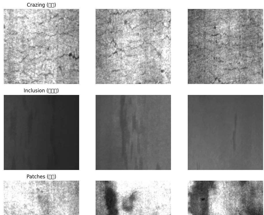
I confirmed that the visual characteristics of each class are clearly different. This is a sign that there’s enough separability for the model to learn from.
4. Data Preprocessing and Augmentation — What’s Special About NDT Data
NDT data generally shows a severe imbalance where normal samples vastly outnumber defective ones. Also, because data collection itself is expensive, data augmentation is used to boost generalization performance.
Augmentation Strategy — Which Transformations Are Safe
The key criterion when choosing augmentations for NDT: don’t distort the intrinsic characteristics of the defect.
| Augmentation type | Suitable for NDT? |
|---|---|
| Rotation / horizontal-vertical flip | ✅ — defects are orientation-independent |
| Slight brightness adjustment | ✅ — simulates lighting condition variation |
| Strong color changes / tone shift | ⚠️ — distorts the visual characteristics of the defect |
| Heavy distortion / large noise addition | ❌ — blurs the essence of the defect |
Why Augmentation Only Makes Sense on the Training Dataset
Even the same training image gets transformed differently every epoch, so effectively the model sees a wider variety of data. That’s why augmentation is applied only to the training set, not to the validation/test sets.
5. Transfer Learning — Reusing ResNet18 Weights
Training a model from scratch requires a huge amount of data. Transfer learning starts from the weights of a model already trained on a large dataset and retrains only the final classifier layer for our specific problem.
This time, I brought in a ResNet18 trained on ImageNet. Since that model has already learned a variety of visual patterns (edges, textures, shape combinations), replacing just the output layer (nn.Linear) with a 6-class version lets it adapt quickly to our data.
Freezing vs Fine-tuning
- Freezing: freeze all the earlier layers (no weight updates), and train only the newly attached classifier. Safe when data is limited.
- Fine-tuning: start from the pretrained weights but train the entire (or a portion of the) network together. Yields bigger performance gains when there’s enough data.
Training Log
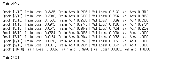
Val Acc reached 1.0 after just 10 epochs. At this stage, the reaction shouldn’t be “great, it worked” but rather “is this really that good, or is it overfitting?” So I plotted the curves to check.
6. Learning Curves — A Machine Learning Engineer’s Basic Skill
Being able to read a learning curve is a basic requirement for a machine learning engineer.
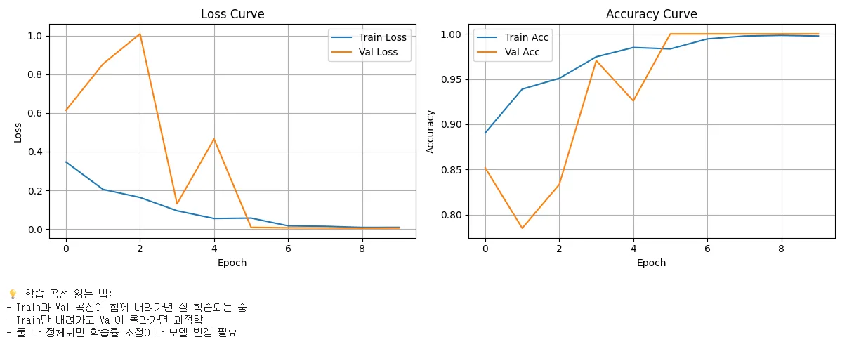
How to read them is actually pretty intuitive.
- If Train and Val decrease together: training is going well
- If only Train decreases while Val increases: overfitting. The model is starting to memorize the training data
- If both plateau: you need to adjust the learning rate or change the model
This time, both curves converged, indicating a normal training pattern. I also revisited my intuition about learning rate: too small, and it takes forever to find the minimum; too large, and it tends to diverge near the minimum.
7. Confusion Matrix — What Matters More Than Plain Accuracy in NDT
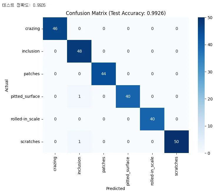
Test accuracy: 0.9926. But in NDT, which classes get confused with which matters far more than plain accuracy. That’s why a Confusion Matrix is essential.
In particular, False Negatives (missing an actual defect) can be the most dangerous, potentially leading directly to safety accidents. False Positives (flagging a defect that isn’t there) cost extra inspection time, but are less critical from a safety standpoint.
But Wait — Why Doesn’t This Matrix Have a “No Defect” Class?
I was confused at first when looking at the Confusion Matrix — I didn’t see any cases of defects being classified as normal. When I looked into it, there was a reason.
Real-world NDT systems typically use a two-stage pipeline:
- Determine defect presence/absence (binary)
- Classify the defect type (multi-class)
The NEU dataset I worked with is a stage-2 dataset. In other words, it’s a model for determining which of the 6 types a defect is, assuming a defect is already present. That’s why there’s no “normal” class at all, and False Negative cases don’t appear in the matrix.
Once I understood this structure, the meaning of 99.26% accuracy became more narrow. It only means “given that a defect is present, the type is classified almost perfectly” — it’s a separate matter from the reliability of stage 1 (presence/absence detection).
8. Grad-CAM — Where Did the Model Look When Making Its Decision?
For an NDT system to be adopted in practice, a simple classification result isn’t enough. Inspectors and regulatory bodies want to see “why the model made this judgment.” The standard tool for this is Grad-CAM.
Grad-CAM is a technique that visualizes as a heatmap which part of the image the model mainly looked at when making a classification decision.
(Similar techniques include SHAP and others — the field of model interpretability has several different branches of tools.)
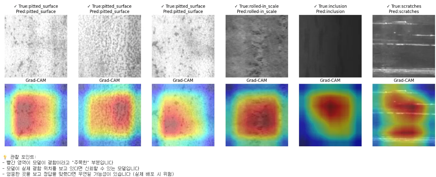
Looking at the heatmap, the model is precisely focused on the defect region. If the model had instead been activated on the image edges or background, it would have suggested a “lucky guess.” Grad-CAM is a verification tool that catches this.
9. Model Saving and Inference Performance
Finally, I saved the model and measured its file size and inference speed to gauge feasibility for embedded deployment.
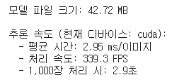
- File size: 42.72 MB
- GPU inference speed: average 2.95ms / image (339.3 FPS)
- Time to process 1,000 images: about 2.9 seconds
This is very fast on GPU, but deploying to an actual embedded environment (edge device / CPU inference) would require additional optimization such as quantization. I didn’t get into the quantization step this time.
Summary
- Transfer learning + data augmentation can achieve ~99% classification accuracy even with limited data.
- In NDT, what matters is not plain accuracy but the pattern in the Confusion Matrix, especially the FN behavior.
- Real-world NDT is a two-stage pipeline (presence/absence detection + type classification) — you need to understand the nature of the dataset to interpret the results correctly.
- Grad-CAM is an essential tool for model adoption — you need to be able to show inspectors and regulators the basis for the model’s decisions.
Things to Study Further
1. Model Quantization
- The tradeoff between accuracy loss and speed/memory improvement with INT8 / FP16 quantization
- PyTorch’s
torch.quantizationworkflow (PTQ vs QAT) - Converting a quantized model to ONNX for deployment on edge devices (Jetson, Raspberry Pi, etc.)
- Reference: PyTorch Quantization Official Guide
2. Building an NDT Two-Stage Pipeline Myself
- Attaching a defect presence/absence binary model in front of this exercise’s classifier to build an end-to-end pipeline
- Training strategies focused on reducing stage-1 False Negatives (class weighting, focal loss, etc.)
- How to measure and manage the overall system’s FN rate when combining stage 1 and stage 2
3. Model Interpretability — Beyond Grad-CAM
- The differences between Grad-CAM, Guided Grad-CAM, and Score-CAM
- Model-agnostic interpretability tools like SHAP / LIME
- The impact of model interpretability on regulatory approval in medical and industrial domains
- Reference: Grad-CAM paper
4. Revisiting Core PyTorch Concepts
Concepts I was familiar with in this exercise but had trouble explaining in detail, organized for review.
- The internal workings of
nn.Linearand weight initialization - Types of loss functions (CrossEntropy, BCE, Focal Loss) — when to use which
- Differences between optimizers (SGD, Adam, AdamW) and criteria for choosing one
- Learning rate scheduling (StepLR, CosineAnnealing, etc.)
- Reference: PyTorch Official Tutorials
5. The NDT Domain — The Practical Workflow of Vision-Based Inspection
- Difficulties in the data collection stage (rare defects, label consistency, environmental variation)
- Commonalities and differences when expanding to domains beyond steel (semiconductor wafers, medical imaging, aircraft components, etc.)
- How camera/lighting setups on the factory floor affect model performance
6. Transitioning from TensorFlow to PyTorch
- Key differences between the two frameworks (static graph vs dynamic graph, eager execution, ecosystem)
- Common sticking points when porting a model written in TF to PyTorch
- Bidirectional conversion via ONNX
Retrospective
Two things became clear through this exercise.
First, even for the same classification problem, the meaning of an evaluation metric changes completely depending on the domain. “99% accuracy” is an impressive number for ImageNet classification, but in NDT it’s just a starting point that raises the question, “So how many FNs are there?”
Second, model interpretability is no longer optional. I directly felt that without tools like Grad-CAM to show the basis for a model’s judgment, adoption in industrial domains is difficult.
The next step is items 1 and 2 from the “things to study” list above — verifying embedded deployment feasibility through quantization, and building a two-stage NDT pipeline myself. That’s where my embedded object recognition experience and this NDT exercise can connect.