
Today I started with axis. If you picture a table as-is, it’s a list of data with two axes. For yearly student grades, year is one axis and grades is the other.
Table of contents
Open Table of contents
Adding an index to a DataFrame
I put Korean, English, and Math scores into a DataFrame using a dictionary. Doing just this tells you what scores exist, but not whose scores they are. So I added an index.
df = pd.DataFrame({
    "국어": [90, 85, 70],
    "영어": [80, 95, 75],
    "수학": [70, 90, 80]
}, index=["민수", "주성", "철수"])

df
Think of pandas as putting a concept called axes into the DataFrame, letting you select the data you put in.
- The index axis is number
0—df.index - The column axis is number
1—df.columns
The reason they’re distinguished by number is that later you’ll need to pass an axis as a number to some function. If you need to give the row as the axis, it’s 0; if the column, it’s 1.
If you print df.axes, you can see the DataFrame’s axes — df.index and df.columns values are returned in that order. Since index comes first, it’s 0, and since columns comes second, it’s 1.
I trusted the axis number at face value and got confused
Once I had this sorted out, I actually tried using axis, and the value was different from what I expected.
df.sum(axis=0)국어 245
영어 250
수학 240
dtype: int64I gave axis number 0, but I got the sum of columns. Doing the opposite gives this:
df.sum(axis=1)민수 240
주성 270
철수 225
dtype: int64I thought axis=0 is the index axis, so I expected per-index totals — but it was exactly the opposite.
Here’s why. axis doesn’t mean “what to group by” — it means “which direction to sweep through.” With axis=0, the calculation sweeps from top to bottom along the row direction, so the data in that direction collapses, leaving the columns behind. With axis=1, it sweeps along the column direction, so the columns collapse and the index remains.
So it’s easier to remember by the length of the result. axis=0 gives a result with as many entries as there are columns, and axis=1 gives a result with as many entries as there are rows.

The place you’ll actually use this most is when deriving a new column.
df["총점"] = df.sum(axis=1)Since you need one value per row for it to attach to the new column properly, this is axis=1.
If the axis really gets too confusing, you can also transpose the DataFrame with transpose and work from there. But since this can be heavy for large data, it’s lighter to attach head(1) just to check the direction.
df.head(1).TPulling out exactly the data you want with loc
When presenting data, you should assume you’re showing it to someone without domain knowledge. For those people, visualization improves readability. To do that, you need to be able to build a table and pull out only the data needed for visualization.
Like a Series, a DataFrame can also be accessed with loc, which looks things up by label.
orders.loc["O002"]order_date 2026-08-02 00:00:00
customer 서연
region 부산
product 모니터
quantity 1
unit_price 320000
paid True
total_amount 320000
Name: O002, dtype: objectIf you give loc a single value, it’s interpreted as a row label. But sometimes you only want to know, say, the customer name from the row you found. In that case, give a column label after the row label.
orders.loc["O002", "customer"]

# Output: '서연'
If you think of position in matrix terms, it’s not (x, y) as on a coordinate plane but (y, x) order. It’s easier to think of an array as a table, not a coordinate system.
Getting multiple rows
Since you’re picking multiple rows, you pass an array into loc.
orders.loc[
    ["O002", "O004"]
]
When I selected a single row, it came out as a Series, but selecting two gives a DataFrame. However, even if you select just one, you can still get a DataFrame back by wrapping it in an array. Getting a Series gives you 1D, getting a DataFrame gives you 2D, and each has its own use.
If you need multiple rows and multiple columns, give each as an array.
orders.loc[
    ["O002", "O004"],
    ["order_date", "customer"]
]
Slicing
Slicing worked on a Series, and it works on a DataFrame too.
orders.loc["O001":"O004"]It naturally works on rows, and it works on columns too. So I wondered whether you could slice or select only columns without applying anything to the rows — and you can, by giving : in the row position.
orders.loc[:, ["customer", "total_amount"]]: means “all rows.” This helps when you want to cut out and view only the data you want.
iloc — position-based
There’s also a way to index by position instead of label.
orders.iloc[0]iloc can also take an array.
orders.iloc[
    [0, 2, 4]
]
Position-based slicing also works.
orders.iloc[1:4]But this kind of slicing behaves exactly like Python’s array slicing, so it does not include the last index. loc does include it, so you shouldn’t get the two confused. This is the same thing that tripped me up when I looked at Series in a previous post — and it’s the same for DataFrames.
Besides loc, there’s also at. It’s not exactly the same, though — at is meant for pulling out a single value only. You can’t pass slices or arrays into it, but in exchange it’s that much faster.
Filtering by condition
Now, filtering. I first looked at picking out only the data whose values satisfy some condition. Filtering uses a boolean mask.
Conditions are usually set based on a column. You pick one column from the DataFrame to build the condition on, pull it out as a Series, and apply the condition to that Series to create the mask.
condition = orders["quantity"] >= 2

orders[condition]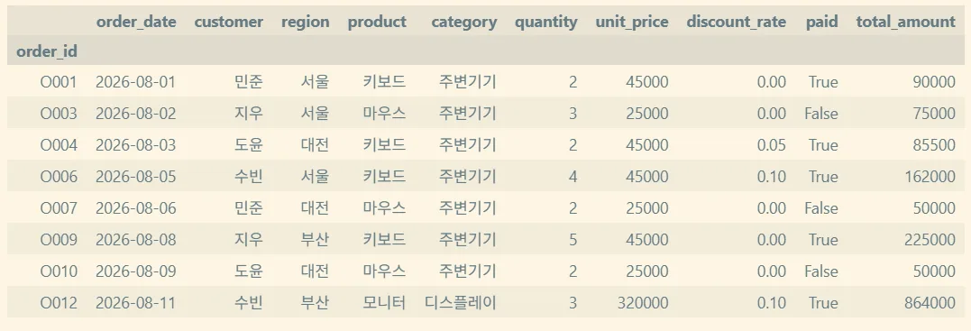
Only the True rows satisfying the condition are printed, and the rest are excluded.
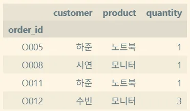
Not just inequality operators — Python comparison operators like == work the same way when building a condition expression. And you can also pick out specific columns from the filtered result.
filtered = orders[orders["total_amount"] >= 300000]

filtered[
    ["customer", "product", "quantity"]
]
If you want to use two or more conditions, use & or | just like you did with a Series.
orders[
    quantity_condition & total_condition
][["product", "quantity"]]
This way, you can pull out data satisfying a condition and narrow it down to only the columns you need to show.
If results like this can be based on 5 or 10 years of accumulated data, customer-tailored marketing also becomes possible. But what matters here is domain knowledge. Without domain knowledge, even if you look at the data, you can’t extract insight. You need to understand the domain to see why transshipment takes so long, or what data to pay attention to in maritime logistics.
The order of data exploration
At the end of the lecture, we went over the order to follow when first examining a DataFrame.

1. Check that the data loaded correctly
df.head()2. Check the size (shape) of the data
df.shape3. Check the columns and index
print(df.columns.to_list())print(df.index.to_list())
# print(df.index) # when the index is a plain RangeIndex4. Check the data types
print(df.dtypes)5. Check the overall structure
print(df.info())6. Check for missing values
You should be able to count how many missing values each column has.
df.isna().sum()axis applies here too. If you give nothing to sum(), the default is axis=0, so you get the count of missing values per column.
7. Check descriptive statistics (distribution of numeric data)
Descriptive statistics are only meaningful for numeric data.
df[select_cols].describe()
# You can also just call df.describe() directly,
# but it's better to exclude categorical data first.
8. Check categorical data
For categorical data, what’s actually in it matters. If something is supposedly categorical but has 100 distinct values, calling it a category doesn’t mean much.
df["species"].unique()
# Prints only the unique values among categorical data
If you want to see the count, use nunique(). And finally, check how many of each category there are.
df["species"].value_counts()

# df["species"].value_counts().sort_index()
# also sorts the result.
9. Sampling
I already did head() earlier, but it’s also good to do a simple sampling. head() only shows the front, so if something strange exists toward the end or in the middle, it won’t catch it.
df.sample(n=5, random_state=42)Summary
axisisn’t “the grouping basis,” it’s “the sweep direction.” It’s less confusing to remember it by the length of the resultlocis label-based,ilocis position-based. When slicing,locincludes the end,ilocdoesn’t- If you want to keep all rows and select only certain columns, give
:in the row position - Filtering means building a boolean mask with a condition expression and applying it to the DataFrame
Things to study further
- The difference between
at/iatandloc/iloc— In my notes I wrote thatatfunctions the same asloc, but checking further,atturned out to be only for accessing a single value. I want to see when the speed difference actually becomes meaningful. → pandas: Fast scalar value getting and setting SettingWithCopyWarning— This warning appears when you assign a value into a filtered result. I understand it depends on whether the filtered result is a copy or a view of the original, but I don’t fully understand it yet. → Returning a view versus a copy- The
query()method — Apparently, when you have multiple conditions, you can write them as a string instead ofdf[cond1 & cond2]. I want to compare how much it improves readability. → DataFrame.query describe(include="all")— An option that produces descriptive statistics including categorical data. I’m curious whether it can replace step 8 entirely. → DataFrame.describe- numpy’s axis — pandas’
axisultimately comes from the numpy concept. I think looking at how axes work once you get to 3+ dimensions will help clear up what’s confusing me now. → NumPy: axes